
Today we discuss how to handle big data with Excel. This article is for marketers such as brand builders, marketing officers, business analysts and the like, who want to be hands-on with data, even when it is a lot of data.
Why bother dealing with big data?
If you are not the hammer you are the nail. We, the marketers, should defend our role of strategic decision-makers by staying in control of the data analysis function that we are losing to the new generation of software coders and data managers. This requires us to improve our ability to deal with large datasets, which may have several benefits. Perhaps the most appealing one from a career standpoint is to reaffirm our value in the new world of highly-engineered, relentlessly growing and often inflexible IT systems, filled with lots of data someone thinks could be very useful if only appropriately analyzed.
To this extent many IT departments are employing Data Architects, Big Data Managers, Data Visualizers and Data Squeezers. These programmers, specializing in different kinds of software, are in some cases already bypassing collaboration with the marketers and going straight into the development of applications used for business analytics purposes. These guys are the new competitors to the business leader role, and I wonder how long it will take until they begin making the strategic decisions too. We should not let this happen, unless we like being the nail!
Hands-on big data with Excel
MS Excel is a much loved application, someone says by some 750 million users. But it does not seem to be the appropriate application for the analysis of large datasets. In fact, Excel limits the number of rows in a spreadsheet to about one million; this may seem a lot, but rows of big data come in the millions, billions and even more. At this point Excel would appear to be of little help with big data analysis, but this is not true. Read on.
Consider you have a large dataset, such as 20 million rows from visitors to your website, or 200 million rows of tweets, or 2 billion rows of daily option prices. Suppose also you want to investigate this data to search for associations, clusters, trends, differences or anything else that might be of interest to you. How can you analyze this huge mass of data without using cryptic, expensive software managed by expert users only?
Well, you do not necessarily have to – you can use data samples instead. It is the same concept behind common population survey. to investigate the preferences of adult males living in the USA, you do not ask 120 million persons; a random sample can do it. The same concept applies to data records too, and in both cases there are at least three legitimate questions to ask:
-
- How many records do we need in order to have a sample we can make accurate estimates with?
- How do we extract random records from the main dataset?
- Are samples from big datasets reliable at all?
Try LogRatio’s fully automated solution for the professional analysis of survey data.
In just a few clicks LogRatio transforms raw survey data into all the survey tables and charts you need,
including a verbal interpretation of the survey results.
It is worth giving LogRatio a try!
How large is a reliable sample of records?
For our example we will use a database holding 200,184,345 records containing data from the purchase orders of one product line of a given company during 12 months.
There are several different sampling techniques. In broad terms they divide into two types: random and non-random sampling. Non-random techniques are used only when it is not possible to obtain a random sample. And the simple random sampling technique is appropriate to approximate the probability of something happening in the larger population, as in our example.
A sample of 66,327 randomly selected records can approximate the underlying characteristics of the dataset it comes from at the 99% confidence interval and 0.5% error level. This sample size is definitely manageable in Excel.
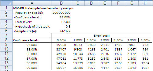
Image 1: Random sample sizes produced with the bernoullian formula
according to population size, confidence interval and error level.
The confidence level tells us that if we extract 100 random samples of 66,327 records each from the same population, 99 samples may be assumed to reproduce the underlying characteristics of the dataset they come from. The 0.5% error level says the values we obtain should be read in the plus or minus 0.5% interval, for instance after transforming the records in contingency tables.
How to extract random samples of records
Sampling statistics is the solution. We used the tool Sample Manager of MM4XL software to quantify and extract the samples used for this document. If you do not have MM4XL, you can generate random record numbers as follows:
-
- Enter in Excel 66,327 times the formula =RAND()*[Dataset size]
- Transform the formulas in values
- Round the numbers to no decimals
- Make sure there are no duplicates [2]
- Sort the range and you get a list of numbers as shown in the following image
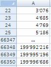
Extract these record numbers from the main dataset: This is your sample of random records. The number 3,076 in cell A22 shown above means that record number 3,076 of the main dataset is included in the sample. To reduce the risk of extracting records biased by the lack of randomness, before extracting the records of the sample, it is a good habit to sort the main list, for instance alphabetically by the person’s first name or by any other variable that is not directly related to the values of the variable(s) object of the study.
If we are ready to accept the approximation imposed by a sample, we can enjoy the freedom of being hands-on with our data again. In fact, although 66,327 records can be managed fairly well in Excel, we still have a sample large enough to uncover tiny areas of interest.
Large sample sizes enable us to manage very large datasets in Excel, an environment most of us are familiar with. But what is the reliability of such samples in real life?
Are samples extracted from big data with Excel reliable at all?
The key question is: Can a random sample reproduce accurately enough the underlying characteristics of the population it is extracted from? To find some evidence we:
-
- Measured several characteristics of our whole dataset, the underlying population.
- Then we extracted random samples from the main dataset and we measured the same characteristics as for the whole dataset.
- Finally we ran several confirmatory tests comparing the measurements conducted on both samples and main dataset.
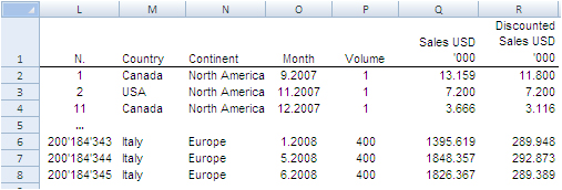
The image below shows the fields of our records. They can be read as follows: Record number 1 (row 2) is a purchase order from North America, received on September 2007, concerning one single item priced USD 13,159 and sold for USD 11,800.
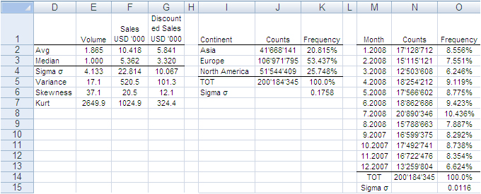
The next image shows the measures computed on the single variables. The Average and Median value were computed for the fields “Volume”, “Sales” and “Discounted Sales” (see range D1:G3). Counts and Count Frequencies were found for the variables “Continent” (see range I1:K4) and “Month” (see range M1:O13). For instance, 1.865 in cell E2 stands for the average number of items in one purchase order. USD 5,841 in G2 stands for the average selling price of one sold item. In K2, 20.815% is the share of items (products) sold to Asia and, in O2, 8.556% is the share of items sold during January 2008. We will test whether random samples can approximate the average values and the percent frequencies shown in the following image.
In accordance with the ASTM manual[1], we drew 20 randomly selected samples of 66,327 records each from the population of 200,184,345 records. For each sample we computed the same values shown in the image above and to each value we applied a Z-test to identify any anomalous values in the samples. The Z-tests were run for both continuous and discrete variables.
All-in-one, continuous metrics
The next table shows test results for the variables “Volume”, “Sales” and “Discounted Sales”. Cell B1, for instance, tells us on average one purchase order (a record) of the main dataset accounts for a sales “Volume” equal to 1.865 items with an “Average Sales” value of USD 10’418 and an “Average Discounted Sales” value of USD 5’841. For sample values departing severely from the control values in row 2 the probability is high that a Z-test at the 99% probability level captures the anomaly.
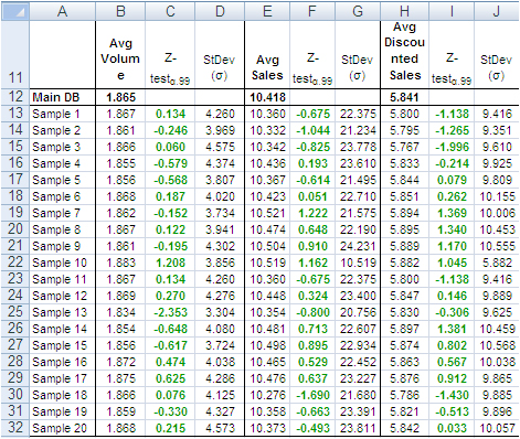
According to the “Z-Test” columns of the image above, no one single sample reports average values different from the averages of the main dataset. For instance, the “Average Volume” of Sample 3 and that of the main dataset differ only by 0.001 units per purchase order, or a difference of about 0.5%. The other two variables show a similar scenario. This means that Sample 3 produced quite accurate values at the global level (all records counted in one single metric).
Categorical metrics
We tested the variable “Continent”, which splits into three categories: Asia, Europe and North America. Columns B:D of the following table show the share of orders coming from each continent. The data in row 15 refer to the main dataset. In this case too, the difference between main dataset and samples is quite small, and the Z-Test (columns E:G) shows no evidence of bias, with the exception of slight deviations in Europe for sample 5, 8, 9, and 18-20.
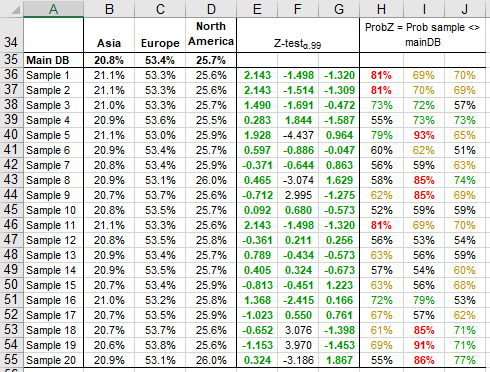
The “Probability” values in column H:J measure the likelihood a sample value is different from the same value of the main dataset. For instance, 21.1% in B36 is smaller than 20.8% in B35. However, because the former comes from a sample, we need to verify from a statistical point of view the probability the difference between the two values is caused by a bias in the sampling method. The 95% is a common level of acceptance when dealing with this kind of issue. With small sample sizes (30), the 90% probability threshold can still be used, although this implies higher risk of erroneously considering two values equal when in fact they are different. For the sake of test reliability we worked with the 99% probability threshold. In H36 we read the probability B36 is different from B35 equals 81%, the very beginning of the area where anomalous differences can be found. Only the share of Sample 5 and 19 for Europe is above 90%. All other values lie well away from a worrying position.
This also means that the share of purchase orders incoming from the three continents reproduced with random samples do not show evidence of dramatic differences outside the expected boundaries. This can also be intuitively confirmed simply by looking at the average sample values in the range B36:D55 of the above image; they do not differ dramatically from the population values in the range B35:D35.
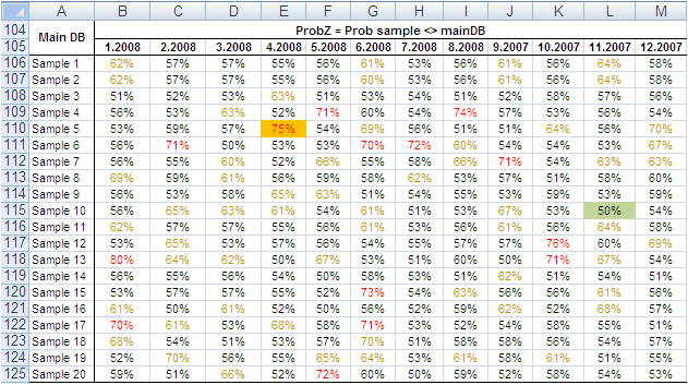
Finally, we tested the variable “Month”, which splits into 12 categories and therefore could generate weaker Z-Test results due to the shrinking size of the sample by category. Columns B:M in the following table show the probability that the sampled number of purchase orders by month differs from the same value from the main dataset. No one sampled value is different from the correspondent value from the main dataset with a probability larger than 75% and only a small number of values have a probability larger than 70%.
The results of the tests conducted on all samples did not find severe anomalies that would discourage the application of the method described in this paper. The analysis of big datasets by means of random samples produces reliable results.
Can the reliability of this Experiment have happened by chance?
So far, the random samples have performed well in reproducing the underlying characteristics of the dataset they come from. To verify whether this could have happened by chance, we repeated the test using two non-random samples: the first time taking the very first 66,327 records of the main dataset and the second time taking the very last 66,327 records.
The results in short: out of 42 tests conducted with both discrete and categorical variables from the two non-random samples, only three had green Z-Test values. That is, these three sample values were not judged different from the same value from the main dataset. The remaining 39 values, however, lay in a deep red region, meaning they produced an unreliable representation of the main data.
These test results too support the validity of the approach by means of random samples, and confirm that the results of our experiment are not by chance. Therefore, the analysis of large datasets by means of random samples is a legitimate and viable option.
Closing
This is a great time for fact-and-data driven marketers: There is a large and growing demand for analytics, but there are not enough data scientists available to meet it yet. Statistics and software coding are the two areas we should deepen our knowledge of. At that stage a new generation of marketers will be born, and we look forward to their contribution to the relentless evolving world of brand building. Software tools like MM4XL can help us along the way because they are written for business people rather than statisticians. Such tools should become a key component of our toolbox for generating insights from data and making better business decisions.
____________________________________________
[1] Manual on the Presentation of Data and Control Chart Analysis, 7th edition. ASTM International, E11.10 Subcommittee on Sampling and Data Analysis.
[2] My sincere thanks to Darwin Hanson, who caught a couple of issues: (1) RND is a VBA function, and I meant of course the spreadsheet function RAND; and (2) you must double-check the random numbers and get rid of duplicates.