Contingency tables are also called cross tables or crosstabs because they actually present the crossed counts of two or more variables.
Anatomy of a cross table
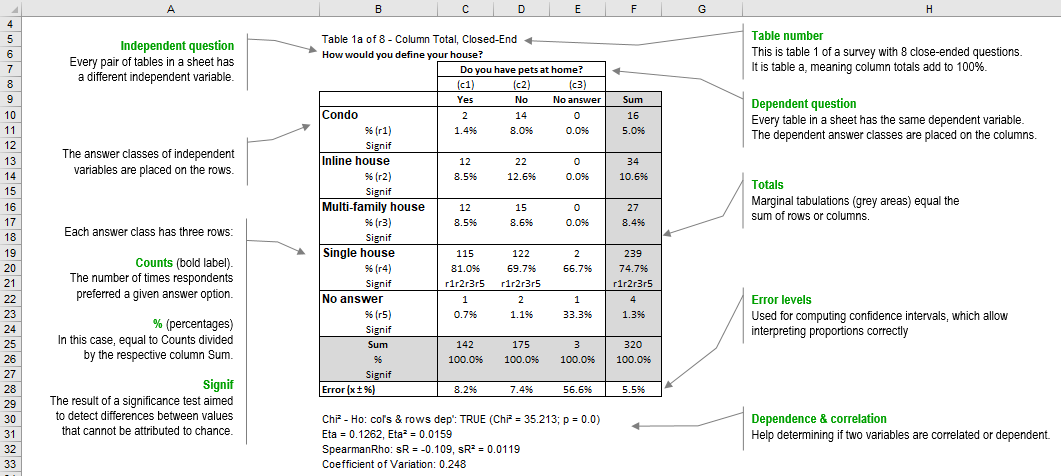
Image 2: How to read crosstabs
The cross tables LogRatio makes are also called two-way tables because they are made with the crossed answer classes of two questions: one as the column and the other as the row.
In LogRatio’s tables each answer class has three rows of information called: Counts (bold label), % (percentages), and Signif. The totals (Sum), also called Marginal tabulation, follow the same rule with three rows. The error levels complete the picture.
The text that follows explains each element of LogRatio’s cross tables in detail.
Counts
This is the number of times respondents preferred a given answer option to a survey question. For instance, in our example, out of 320 answers, 239 respondents answered question “How would you define your house” with “Single house”; of these, 115 respondents have pets at home, 122 don’t, and 2 did not answer this question.
Percentages
Counts are converted to percentages, to help the analyst in figuring out the proportions between sub-groups of respondents. Proportions, or percentages, are important because they can lead to identifying groups or clusters of respondents with common characteristics, they help in prioritizing, and, very important, percentages enable testing the significance of their differences.
In our example, 74.7% (or 239) of the 320 respondents answered “Single house” to question “How would you define your house”. 81.0% (or 115) of the 142 respondents with pets at home also answered “Single house”.
The percentages of table A are made from column totals, while in table B (see image 1 in the previous section) the percentages are computed on row totals. These two views are able to uncover a lot of information.
Significance test
Testing the significance of the difference of two proportions makes sure the proportions are not just the result of variation by chance.
LogRatio uses the Z-test at the 95% confidence level to compare the significance of the differences between proportions of crosstabs, and when it finds a significant difference, LogRatio adds a string on the relevant row Signif.
For instance, cell C21 in the image above shows “r1r2r3r5”, which means: 81% is a value statistically larger (not due to chance) than the other proportions in row 1, 2, 3, and 5 of answer class c1 (see row 8 of image 2). These are: 1.4% (r1 = row 1 of the table), 8.5% (r2 and r3 = row 2 and 3 of the table), and 0.7% (r5 = row 5 of the table).
The table above has column totals. Tables with row totals replace the r with a c, for column, and are read horizontally instead of vertically as in this example (see table B of image 1 in the previous section).
Error levels
Error levels are perhaps the most critical elements to interpret correctly the data of a cross table.
In the Sample size section of its report LogRatio computes the overall error level of the survey, 5.5% in our example (repeated in cell F28 of the table above). This means, for instance, that the 10.6% in cell F14 should be read as “any value in the interval 10.6% ±5.5%”, that is any value between 5.1% and 16.1%. This overall error value is found using the whole sample size (320 respondents in our example), therefore it applies only to the total (Sum) proportions of a table, both row and column totals.
Reading a proportion in the white area of the table above requires computing the appropriate error level based on the relevant sample size. The proportion 8.5% of cell C14, for instance, should be read as “any value in the interval 8.5% ±8.2%” according to the sample of 142 respondents as in cell C25.
In this example, row 28 holds the error levels by column for table A. Table B holds, in its last column, the error levels by row.
Variables dependence and correlation
Under table A of each pair of tables LogRatio prints several coefficients useful for finding out whether the two variables are dependent or correlated.
Chi squared test
Dependent variables are linked by a relationship, and this relationship can be tested with a Chi2 test. The result of the independence test reads like this: “Chi2 – Ho: col’s & rows dep’: TRUE (Chi2 = 125.837; p = 0.0)”.
If the variables are independent the Chi2 test results FALSE. If they are related the test returns TRUE. The p-value supplies the confidence level of the test, where: (p less or equal to 0.05) = TRUE.
Correlated variables tend to move together. That is, high values of variable A tend to correspond to high or low values of variable B. This is not causation, we cannot say one variable causes the other, but we can still spot dynamics that can lead to concrete actions. For instance:
- Dynamic: The quantity of toothpaste used correlates to smoking habits: smokers use less.
- Action: Consider educating smokers to use more toothpaste of brand X.
LogRatio’s tables supply the Eta and the Spearman’s Rho Correlation Coefficient, both also squared, to measure the relationship that characterizes the two variables.
Eta correlation coefficient
Eta, the coefficient of nonlinear relationship, is often useful to measure a relationship irrespective of if it is linear or not. Eta suits the case of categorical variables, it is interpreted similarly to the Pearson, but can never be negative.
The Eta Correlation Coefficient is an index ranging from 0 to 1.0 and reflects the extent of a nonlinear relationship between two data sets. Eta squared tells us more about the strength of the relationship between variables, it measures the proportion of variation explained by the independent variable. In the case of the table above both values are very low (Eta = 0.1262, Eta squared = 0.0119) signifying a lack of correlation between pets at home and house kind.
Spearman’s Rho
Rho measures the strength and direction of the association between two ranked variables. It ranges from -1 to 1, where negative values show an increasing negative correlation and positive values show an increasing positive one.
In the case of the table above both values are very low (Rho = -0.109, Rho squared = 0.0119), which suggests a very low negative correlation between pets at home and house kind. In fact, only 1.19% (Rho squared) of the variation in the dependent variable pets at home can be explained with the variable house kind.